Visualizing motion capture in Matlab

MocapTools was released in our paper for automated gap filling for marker-based biomechanical motion capture data. In the paper we showcased MocapTools and studied the main feature of gap filling with validation using inverse kinematics.

Here is the bibtex reference if you want to cite:

@article{doi:10.1080/10255842.2020.1789971,
author = {Jonathan Camargo and Aditya Ramanathan and Noel Csomay-Shanklin and Aaron Young},
title = {Automated gap-filling for marker-based biomechanical motion capture data},
journal = {Computer Methods in Biomechanics and Biomedical Engineering},
volume = {23},
number = {15},
pages = {1180-1189},
year  = {2020},
publisher = {Taylor & Francis},
doi = {10.1080/10255842.2020.1789971},

There are many features in MocapTools that could be helpful for Biomechanics research. In a series of posts I will highlight them, showing some examples of use. This post will cover the visualization of marker data.

You can use MocapTools to visualize marker data in two ways:

1) Load and plot marker trajectories in time.

2) Plot skeletons and markers by using the definition of a vsk file.

In motion capture, the standard format is the C3D file. This contains all the information recorded in a session. Vicon Nexus saves files in the native format but after reconstructing and saving the data it will generate C3D files for each trial. When you learn to use Nexus, the typical workflow is to export each data type as csv files. This is redundant, as your C3Ds already contain all the information you need and it can be loaded easily in Matlab.

With MocapTools, You can read marker data using Vicon.C3DtoTRC. By default, all the coordinates are exported using the OpenSim convention with the y-axis pointing up in the vertical direction. If you want to transform the coordinate frames use Vicon.transform.

%% Read the marker data into a table (Header column contains the time in s)
trc=Vicon.C3DtoTRC('SampleFiles\speed_0_5.c3d');
trc{:,2:end}=Vicon.transform(trc{:,2:end},'ViconXYZ'); %transform from Osim (default) to Vicon coordinates

You can also read the forceplate data with Vicon.C3DtoMOT. Here I’m also using Vicon.transform to get the data in Vicon coordinates with the z axis pointing up. I’m also reading the position of the forceplates in the C3D file with Vicon.ExtractCorners. This function gets the corner points of the forceplates.

%% Read the forceplate data and location of forceplates
fp=Vicon.C3DtoMOT('SampleFiles\speed_0_5.c3d');
fp{:,2:end}=Vicon.transform(fp{:,2:end},'ViconXYZ'); %transform from Osim (default) to Vicon coordinates
fpLocations=Vicon.ExtractCorners('SampleFiles\speed_0_5.c3d');
fpLocations.FP1{:,2:end}=Vicon.transform(fpLocations.FP1{:,2:end},'ViconXYZ'); %transform from Osim (default) to Vicon coordinates
fpLocations.FP2{:,2:end}=Vicon.transform(fpLocations.FP2{:,2:end},'ViconXYZ'); %transform from Osim (default) to Vicon coordinates

In the trc variable you can find X,Y,Z coordinates for each marker in the c3d file. You can plot any marker by accessing the column by its name or index. Make sure to check the help for Matlab tables if you are not familiar with the curly brackets and dot notation. If you want to have separate data structures for each marker, instead of Vicon.C3DtoTRC you can use Vicon.ExtractMarkers. This data structure splits every marker on its own field. With it, you can use the tools from EpicToolbox to manipulate individual marker data, instead of having a table with the entire marker positions. Let’s save that for a future post, for this example, I will keep working with the Vicon.C3DtoTRC output.

%% Plot as a time series
figure(1);
subplot(1,3,1);
plot(trc.Header,trc.LASIS_x);
xlabel('Time (s)'); ylabel('LASIS_x (mm)');

subplot(1,3,2);
plot(trc.Header,trc.LASIS_y);
xlabel('Time (s)'); ylabel('LASIS_y (mm)');

subplot(1,3,3);
plot(trc.Header,trc.LASIS_z);
xlabel('Time (s)'); ylabel('LASIS_z (mm)');

Time series of LASIS marker position

Now plot the 3D trajectory of the marker using Matlab’s plot3. I’m also including a plot of the perimeter of the forceplates so that the 3D space is easier to interpret visually. If you plot the sample data, you will see some markers’ trajectory when walking on a treadmill.

%% Plot marker trajectory in time and location of forceplates
fp1points=[reshape(fpLocations.FP1{1,2:end},3,4) fpLocations.FP1{1,2:4}'];
fp2points=[reshape(fpLocations.FP2{1,2:end},3,4) fpLocations.FP2{1,2:4}'];

figure(1);
plot3(trc.LASIS_x,trc.LASIS_y,trc.LASIS_z,'b'); hold on;
plot3(trc.RASIS_x,trc.RASIS_y,trc.RASIS_z,'r'); 
plot3(trc.LLKNEE_x,trc.LLKNEE_y,trc.LLKNEE_z,'b'); 
plot3(trc.RLKNEE_x,trc.RLKNEE_y,trc.RLKNEE_z,'r'); 
plot3(trc.LLTOE_x,trc.LLTOE_y,trc.LLTOE_z,'b'); 
plot3(trc.RLTOE_x,trc.RLTOE_y,trc.RLTOE_z,'r'); 
plot3(fp2points(1,:),fp2points(2,:),fp2points(3,:),'b'); 
plot3(fp1points(1,:),fp1points(2,:),fp1points(3,:),'r'); hold off;
xlabel('x (mm)'); ylabel('y (mm)'); zlabel('z (mm)');

Time series of LASIS marker position

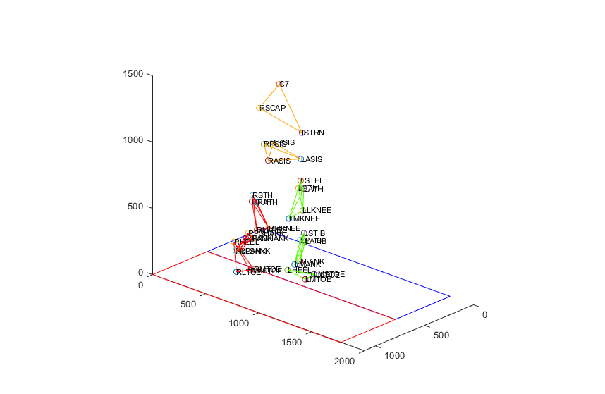
Visualizing trajectories is helpful but it’s not as good as looking at the entire markerset. MocapTools includes functions to read a VSK file that contains the marker skeleton information and also plot the markers using that data. For example, plotting the 100th frame of the capture can be done in a line of code. A pro tip: you can put Vicon.model.plot inside a for loop to create animations.

%% Plot using vsk
figure(1); clf;
Vicon.model.plot('SampleFiles\TFSubject.vsk',trc(100,:)); hold on;
plot3(fp2points(1,:),fp2points(2,:),fp2points(3,:),'b'); 
plot3(fp1points(1,:),fp1points(2,:),fp1points(3,:),'r'); hold off;
daspect([1 1 1]);

Time series of LASIS marker position

That’s all for this post. Feel free to reach out on twitter @jcamargo_co if you need more information!